90-Inch Prime Focus Corrector

Lens 1 Testing Report

Michael Tuell - Optical Sciences Center, University of Arizona, Tucson, Arizona 85716

August 9, 2001

Abstract

This report details the test methods and results for lens 1 of the 90PFC system. It was found to not quite meet specifications in a transmission test configuration.

Table of Contents

Abstract Summary Appendix A: System vs. lens tolerances Appendix B: Testing system tolerance analysis Appendix C: Testing system alignment procedures Appendix D: Test results Appendix E: Testing system photographs Appendix F: Testing system Zemax analysis

1 2 4 5 8 9 11 14

Summary

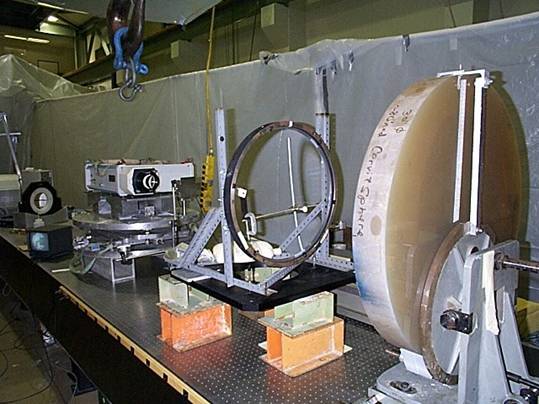
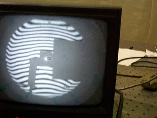
Lens 1 for the 90PFC is an approximately 20” diameter meniscus lens made of fused silica. It was tested in double-pass transmission mode with a spherical return mirror. Figure 1 shows the test system layout. The distance from the interferometer focus (at the right side of the figure) to the vertex of the return sphere was 1.726 meters. An f/1.5 transmission sphere was used as the reference in the interferometer.

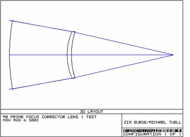
Figure 1

A laser-based Fizeau phase-stepping interferometer was used at 632.8 nm.

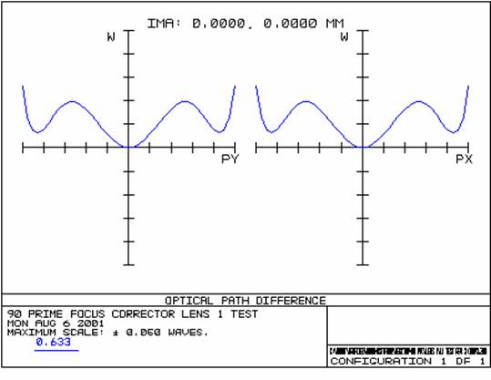
The return sphere was measured and subtracted from the transmitted wavefront map. The lens was measured to be 0.1085 waves rms and has an average slope of 0.0276 waves/cm, whereas from the lens specification, the tolerance is 0.0266 waves/cm.

Figure 2 final wavefront map

Figure 2 shows the final transmitted wavefront over a 480 mm aperture after subtraction of the return sphere, median filtering and a small amount of slope clipping.

The outside diameter of the optic was measured to be 520 mm and the optic weighs about 37 pounds.

The test tolerances show that the rms error could be 0.0093 waves, which is much smaller than the reported error, implying that this data is not swamped out by errors inherent in the test and/or alignment.

Appendix A: System vs. Lens Tolerances

By inspecting the system tolerance budget in Jim Burge’s system tolerancing report from 9/1/99 and comparing them to lens 1, we can find an average ratio, which relates rms spot size to rms slope. Table A1 relates the physical parameters of lens 1 to rms spot radius.

System Parameter RMS spot radius (mm)

Surface 1	0.001089
Surface 2	0.000757
Index homogeneity	0.001027
Root Sum Square total	0.001677

Table A1

The PFC specifications are given in terms of rms spot radius, whereas the lens measurements are in terms of rms slope. A conversion factor, derived from the physics of the situation, of 0.063 gives an rms slope of 0.0266 waves/cm.

Appendix B: Testing System Tolerance Analysis

In order to model the opto-mechanical tolerances for the test system, Zemax was used to individually perturb system element locations. The rms wavefront changes from each perturbation were then added together by the root sum square method. Each part of the system was carefully measured and the measurement tolerance was used to perturb the system. For example, the distance between the lens and the return sphere was perturbed, introducing spherical aberration. The system (focus) was re-optimized for this new spacing and the rms difference was recorded.

To optimize the system in Zemax, the merit function defines the real lateral ray height to be zero at the focus of the interferometer, with further constraints on the best wavefront. The location of focus was given much more weight than the wavefront shape. To optimize a system, there must be variables for Zemax to change. In this case, the variables were the following items: the longitudinal position of lens 1 (for focus control) and the tip/tilt of the return sphere.

Even with no perturbations in the system, it was still not perfect. In fact, the rms wavefront error was 0.005313 waves. To find the additional rms error introduced by perturbation of a system element, we need to take the rms error reported squared minus the square of the unperturbed rms error and then take the square root of that. This is simply root sum square in reverse.

Table B1 shows the rms error and change from the unperturbed case for each system parameter. All of the perturbations are “as measured” values of alignment tolerances. Each system parameter can only be measured/aligned to within a certain tolerance. These values are those tolerances for the specific metrology or alignment technique used. Each parameter was calculated for both “+” and “–“ directions. If the two errors were different, only the largest one is reported.

Figure B1 is a bar chart showing the relative increase for each perturbation (in rms waves.) The x-axis is the index number listed in Table B1. In all cases, the larger of the two rms errors (either “+” the tolerance or “–“ the tolerance) was chosen for the graph and included in the root sum square calculation of the total error budget.

By taking the root sum square of the additional rms values, we find a total of 0.00744 waves rms. This value is well below the target tolerance of 0.0926 waves rms, which means that if these tolerances are held, the data obtained will be useful in determining if the test lens is within its tolerance budget.

Lens 1 Test System Tolerance Table

Element	Index		RMS (waves)	Additional RMS
		Unperturbed	0.005313	0.0053130
Lens placement	1	Z -0.25 mm	0.009090	0.0073756
LENS 3	2	Theta x +0.02°	0.005569	0.0016691
	3	Y +0.3 mm	0.005419	0.0010666
Root Sum Square				0.009303

Table B1

Measurements

The distance from surface 2 of lens 1 to the return sphere was measured with an inside micrometer set to the appropriate spacing of 606.4 mm. Lens tissue was taped to the surfaces of the micrometer to avoid contacting glass to metal. Transferring the measurement from calipers to the protected micrometer gave an error of a few thousandths of an inch and actually placing the lens gave a few thousandths more, so the value of 0.010” (0.25 mm) was used for the tolerance for this measurement.

Adjusting the centering and tilt of lens 1 was accomplished by looking at the focused spot reflected from each surface. Since the optic was large and concave on both sides (as seen from surface 1,) we were able to see a reflected spot focused along the optical axis for each surface. By placing two cards with holes (1.5-2 mm diameter) at the focal points, we were able to align the lens so that both spots went through the holes. These cards were not placed randomly, however. The focused spot at the interferometer’s transmission sphere gave a reference to the “axis” of the interferometer. By adjusting the two cards such that a bright spot was visible through both holes gave us a line defined by three points which became our optical axis. Please see Figure E3.

To keep the image centered on the CCD camera, the first card was placed near the center of the beam by placing a card at the focus and then removing the transmission sphere. This left a collimated beam with a small spot defining the central axis of the interferometer. The first hole was aligned to this spot. The transmission sphere was replaced and the second hole was aligned to view through the first hole to the bright spot at focus.

This technique worked well and gave very low values for coma, indicating a good alignment. This will only work for a meniscus lens which has centers of curvature toward the interferometer focus. Additionally, the lens must be large enough that light passes by the edges of the cards with enough area to allow a focus to be seen. Please see Figure E6 for some idea of how much of the aperture we were blocking in this example.

To determine the sensitivity of this method, we set up a dial indicator on the side of the lens cell and pushed the entire frame to one side with a large screw bolted to the table. Please see Figure E5. By observing when the spots became visible just at the edges of the holes, we were able to determine how well we were able to align the lens. It turned out that by translating the lens 0.012” the spots became just visible. Additional dial indicators were employed to verify that the lens was not tilting or translating in the longitudinal direction.

Zemax was again used to model this test by making the first surface a mirror and looking at how far away from the axis the spot focuses when the lens is decentered. The hole in question (for surface 1) was 1.5 mm in diameter, so if the spot was originally centered, the spot movement would be 0.75 mm. Zemax reported only 0.5 mm for 0.012” (0.3 mm) of decentration, which may be accurate since the spot may not have been originally centered.

Since there was fairly good agreement for decentration, Zemax was used to model the tilt of the lens to determine how much tilt would result in 0.5 mm of lateral shift in the focal point. This turned out to be about 0.02°.

These tolerances were then used in the full Zemax simulation of the test system to determine the effects of these perturbations.

Appendix C: Testing System Alignment Procedures

Alignment of the test system was accomplished by the methods described in appendix B.

The return sphere was the least convenient component to adjust the position of, so the heights of all components were based on the centerline of the return sphere, which was about 61 cm above the optical table. The return sphere is a 30” diameter concave sphere made of Cervit with a ROC of 80.75”. It is mounted in a Unertl mount with tip/tilt and two horizontal translation directions. Please see Figure E1.

The interferometer was placed on a two-axis translation stage which also has three vertical adjustments for leveling the interferometer. A vertical translation stage was placed on top of the first stage, giving us all three Cartesian degrees of freedom as well as tip/tilt for the interferometer.

The test lens was placed in its cell and attached to the frame provided. Please see Figure E4. The frame had four 80 pitch threaded bolts to adjust it, but it was fairly difficult to use since the axes were coupled instead of independent.

Once the crude position adjustments were made, the procedure outlined in appendix B was used to align the lens to the interferometer, defining an axis. Please see Figure E2. The return sphere was then positioned using the inside micrometer as described.

A return spot was observed and adjusted with the tip/tilt on the return sphere until it coincided with the interferometer focus. Fringes were then observed and adjusted with the sphere to minimize tilt fringes. The focus was finely adjusted with the longitudinal adjustment of the interferometer stage.

Appendix D: Test Results

The “raw” wavefront map of the lens in transmission including the return sphere shows some astigmatism, a rolled edge, and a bump in the middle. This map is shown in Figure D1. It has a P-V range of 1.16 waves and an rms of 0.1672 waves. This is for the full aperture of 495 mm, and not the clear aperture of 480 mm. No median filtering was applied at this point.

Figure D1 “raw” wavefront including return sphere

The surface figure of the return sphere was dominated by astigmatism which is most likely gravity and mounting stress induced. Since the mirror was not moved in its mount, we can subtract the surface map from the wavefront map above. Four fiducial marks were placed on the surface of the sphere and used to translate the surface map to align with the wavefront map for subtraction. Figure D2 shows the surface map of the sphere. Figures D1 and D2 are on the same scale. Removing astigmatism reduces the rms error from 0.098 to 0.036 waves.

Figure D2 return sphere surface map

Subtracting Figure D2 from D1, masking down to 480 mm, applying 7x7 median filtering and clipping off the very highest slopes gives the final map shown in Figure 2. This final wavefront map in Figure 2 is also shown here in Figure D3 as a contour map.

Figure D3 “processed” contour map at 480 mm aperture

Appendix E: Testing System Photographs

Figure E1 Test system as seen from return sphere

Figure E2 Lens, sphere and two cards with holes

Figure E3 Laser beam as seen through two small holes for alignment

Figure E4 Lens 1 mounted in its cell and temporary mounting fixture

Figure E5 Dial indicator and screw for misaligning lens 1

Figure E6 Interference fringes showing areas blocked by cards with holes

Appendix F: Testing System Zemax Analysis

The test system was modeled in Zemax in a double-pass configuration at 633 nm. Appropriate coordinate breaks were inserted to allow perturbations for tolerancing, as detailed in Appendix B.

The optimized (unperturbed) system did not have a perfect wavefront. The rms error was reported as 0.005313 waves. Figure F1 shows the OPD as calculated for the unperturbed system. It has a peak-to-valley error of about 0.028 waves.

Figure F1

Table F1, below, shows the full double-pass test system including coordinate breaks for the lens and the return sphere.

Test System Prescription

Surf OBJ 1 2 STO 4 5 6 7 8 9 10 11 12 13 IMA

Type STANDARD COORDBRK STANDARD STANDARD COORDBRK STANDARD COORDBRK STANDARD COORDBRK STANDARD COORDBRK STANDARD STANDARD COORDBRK STANDARD

Comment FOCUS / TILT LENS 1 UNTILT LENS 1 TILT MIRROR RETURN UNTILT MIRROR TILT LENS 1 LENS 1 UNTILT LENS 1

Radius Infinity - 813 622 - Infinity - 2051 - Infinity - 622 813 - Infinity

Thickness -1074.643 -2.35938e-005 -45 0 0 -606.3907 0 0 0 606.3907 0 45 2.35938e-5 1074.643

Glass SILICA MIRROR SILICA

Diam. 1.21e-5 - 480 494 - 0 - 746.6 - 0 - 494 480 - 0.00193

Conic 0 - 0 0 - 0 - 0 - 0 - 0 0 - 0

Table F1